Multifrequency Lockin Basics
lockin measurement
The lockin technique is generally defined by its use of a reference oscillation for making a narrow-band measurement of some physical process [Dicke-1946].
The physical system is excited or modulated with a sinusoidal signal of frequency  , while a phase-locked reference oscillation at the same frequency is used to demodulate, or determine the systems response to the excitation.
Let us denote the response signal as  .
The lockin multiplies this signal with two unity-amplitude reference oscillations and integrates over time, to give two quadrature components.
.
The lockin multiplies this signal with two unity-amplitude reference oscillations and integrates over time, to give two quadrature components.
If the response signal is an oscillation at the frequency with amplitude  and phase
  ,
,
.
and we perform the integrations over a measurement time window,  , corresponding to an integer number
  times the oscillation period
  , we find
.
The quadratures  and
and  are the Fourier coefficients of the response, at the reference frequency.
Note that at DC, or
are the Fourier coefficients of the response, at the reference frequency.
Note that at DC, or  , the integration gives
  and
and  .
At any non-zero frequency we find the following relation between the quadratures and and the response signal amplitude .
.
At any non-zero frequency we find the following relation between the quadratures and and the response signal amplitude .
The response phase is
.
This response phase is with respect to the phase of the reference oscillation, which has zero phase by definition. It is very useful to represent the response signal as complex number,

We call the absolute value of this complex number the quadrature amplitude
Note that at DC, or , the last equivalence does not hold, and we find  .
.
In the time domain the response signal can then be written,
where  is the complex conjugate of
  . Equivalently
![V(t) = 2 \mathbf{Re} \left[ \hat{V} e^{i \omega t} \right] = 2I \cos(\omega t) + 2Q \sin(\omega t)](_images/math/c7efc46fbefbf6659b6daf6854424088ed38ce66.png)
demodulating multiple frequencies
Lockin measurement at one frequency is straight forward, but what happens when there are two frequencies in the excitation waveform and we want to measure the Fourier coefficients of the response at these two frequencies, and perhaps other frequencies. One could use each excitation frequency as a separate reference, but it is far better to define one global reference for all frequencies. The global reference is possible if you carefully choose the excitation frequencies in a process that we call tuning, in direct analogy to the tuning of musical instruments. Below we explain why one should tune a multi-frequency lockin measurement, and how tuning is done with the MLA™.
The MLA™ will excite a physical system with a waveform consisting of many different frequency components, and simultaneously measure both quadratures of the response (i.e. demodulate) at many frequencies.
We refer to the components of the excitation signal and response signal as tones, each having a frequency, amplitude and phase (or alternatively frequency, and two quadrature amplitudes).
The MLA™ is special in that all tones can be locked to one reference, which is also locked to the measurement bandwidth  , or inverse of the measurement time window
  .
Unlike other multifrequency lockins which are simply many independent lockins in one box (the MLA™ can also run in this mode), the MLA™ uses special digital algorithms to achieve many synchronous lockins, all working off the same reference.
This synchronous mode of operation is achieved by tuning the frequencies of all tones to ensure that they are integer multiples of .
.
Unlike other multifrequency lockins which are simply many independent lockins in one box (the MLA™ can also run in this mode), the MLA™ uses special digital algorithms to achieve many synchronous lockins, all working off the same reference.
This synchronous mode of operation is achieved by tuning the frequencies of all tones to ensure that they are integer multiples of .
The number of tones  in your MLA™ may depend on the particular firmware that you are running, but typically
  .
The amplitude and phase of each drive tone in the multifrequency excitation is set by the user, and each tone can be directed to either or both of the MLA™ output ports.
If you do not wish to drive but only ‘listen’ (measure) a particular frequency, simply set both bits of the output-mask to zero at this tone, or set the output amplitude to zero.
The MLA™ measures (demodulates) the quadrature amplitudes of the response at its input ports, at the frequency of each of the tones.
Any tone can be demodulated at one of the 4 input ports.
.
The amplitude and phase of each drive tone in the multifrequency excitation is set by the user, and each tone can be directed to either or both of the MLA™ output ports.
If you do not wish to drive but only ‘listen’ (measure) a particular frequency, simply set both bits of the output-mask to zero at this tone, or set the output amplitude to zero.
The MLA™ measures (demodulates) the quadrature amplitudes of the response at its input ports, at the frequency of each of the tones.
Any tone can be demodulated at one of the 4 input ports.
The demodulation of the response is done by multiplying each digital sample of the input signal with an appropriate demodulating tone and summing over the measurement time window  , as described above. Thus, plays the role of the time-constant of a traditional lockin. We need a word that refers to the data contained in this time window and we chose the word pixel, because the MLA™ was first used in multifrequency AFM [Platz-2008], where each measurement time window corresponds to one image pixel.
Fourier leakage
When a physical system is driven with a number of pure tones, these tones may affect each other in various ways. If the physical system is perfectly linear the principle of superposition applies: The total response is simply a sum, or linear combination of the individual responses at the frequencies of each drive tone. However, Fourier leakage may affect your ability to demodulate and independently measure the various response tones. Fourier leakage occurs when a tone is not perfectly periodic in the measurement time window. A strong tone will ‘leak’ over in to neighboring frequencies in the spectrum and destroy the measurement of other weaker tones.
A digital lockin samples the signal at discrete times and the quadrature amplitudes are calculated with discrete sums. These sums will be corrupted by Fourier leakage when any of the lockin frequencies and sampling frequency are not commensurate (i.e. do not have a common divisor). Thus, the sampling frequency becomes an ideal reference for all tones in a multifrequency digital lockin. Figure 1 demonstrates the connection between sampling and Fourier leakage.
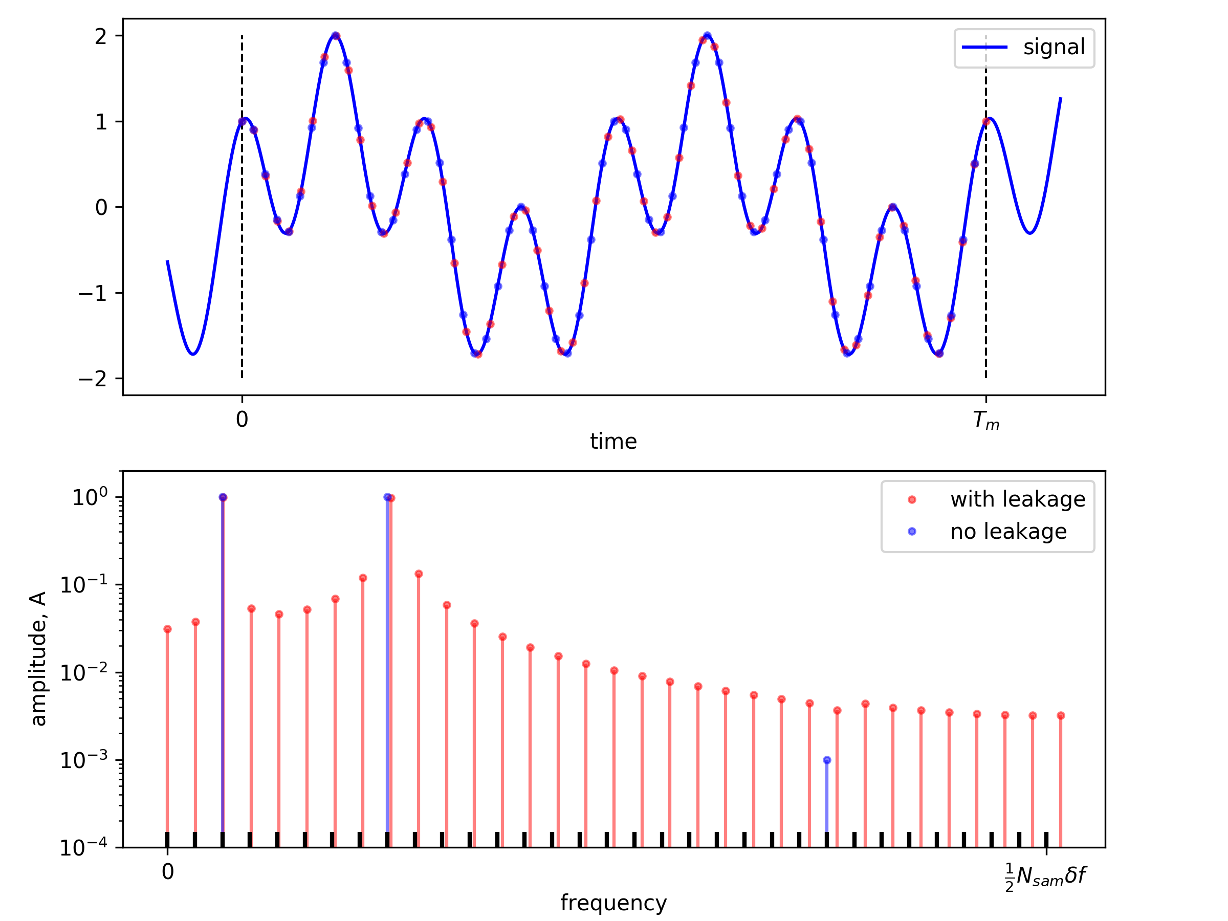
Figure 1: A multifrequency signal with three tones is sampled and Fourier amplitudes are calculated by discrete Fourier sums. The red samples are incommensurate with the frequencies of the tones and the Fourier amplitudes are corrupted with Fourier leakage. The blue samples are commensurate and the spectrum has no leakage, showing amplitude only at the three frequencies contained in the signal. We avoid Fourier leakage by tuning the frequencies of all tones so that they are integer multiples of  , shown by the black grid on the frequency axis.
Fourier leakage can be reduced by so-called windowing, or equivalently, low pass filtering of the demodulated signal, but these methods are imperfect and they can not completely prevent leakage.
To completely avoid Fourier leakage, the MLA™ is designed to work only with frequencies that perform an integer number of oscillations in the measurement time window.
The process of choosing the best frequencies for measurement is called tuning, in analogy to the tuning of musical instruments. The easiest way to tune the MLA™ is to start with a desired measurement bandwidth  and then choose all frequencies to be an integer multiples of .
(1)
where  are a set of integers.
tuning and nonlinearity
Fourier leakage is an issue for the measurement of linear systems, but more fascinating is an effect that occurs in nonlinear systems. A nonlinear system will generate new tones in the response waveform that are not in the drive waveform. Harmonics are generated at exact integer multiples of the drive frequencies and they will occur in nonlinear systems driven with only one tone. Intermodulation products, or mixing products occur when two or more tones are present in the drive, and these occur at frequencies that are integer linear combinations of the drive frequencies. One of the primary design goals of the MLA™ is the accurate measurement of many intermodulation products [Tholen-2011].
When many drive tones are present:  , nonlinear response is generated at very many new frequencies,
(2)
were  are any integer.
Equation (2) tells us that all frequencies in the nonlinear response will be at integer multiples of a base tone  , if we choose the frequencies such that they all have a greatest common divisor . This property of a tonal system in music is referred to as ‘just intonation’ or ‘just temperament’.
The inverse of the base tone  defines the period of the multifrequency waveform. A positive effect of the constraint (1) is that all harmonics and intermodulation products generated by nonlinearity, will also be at frequencies
  , where
  is an integer.
Thus, tuning the measurement also means that the nonlinear response will not be affected by Fourier leakage.
is an integer.
Thus, tuning the measurement also means that the nonlinear response will not be affected by Fourier leakage.
Note that the base tone and the measurement bandwidth are not necessarily the same, but they must have an integer relationship,
(3)
where  is a positive integer.
You can improve the signal-to-noise ratio by reducing the measurement bandwidth while keeping the same base tone (i.e. make
is a positive integer.
You can improve the signal-to-noise ratio by reducing the measurement bandwidth while keeping the same base tone (i.e. make  ). Choosing the base tone to be 2, 3, 4,… times the measurement bandwidth allows you to check for period-doubling, period-tripling, period-quadrupeling,etc., bifurcations in nonlinear response.
setup and tuning functions
When as many as 40 frequencies are involved, setting up the measurement can be a complicated procedure. The MLA™ does have a Graphical User Interface (MLA GUI) with fields for adjusting the drive and reading the response amplitude and phase of each individual tone. But setup and measurement in this manner is often not practical. The MLA™ also has a powerful Application Programming Interface (MLA API) which allows for full setup and control using commands in a Python script. It is simple to edit these scripts and run them directly in the GUI, making for a very flexible environment to set up and test complex multifrequency measurements.
Within the API there are several convenience functions available to facilitate tuning. Tuning functions take a set of target frequencies and a target measurement bandwidth as input arguments. They return a tuned set of frequencies and tuned measurement bandwidth. The set of frequencies can be an entire array of values, or a single ‘carrier frequency’, around which you might build a frequency comb.
The tuning functions behave according to the following rules:
f, df = mla.lockin.tune0(f, df)performs only the minimum about of tuning necessary to make the requested numbers fit the corresponding digital registers in the MLA™ hardware. No attempts are made to avoid Fourier leakage. This function should be used together with a user-defined tuning algorithm, or in rare cases where Fourier leakage is known not to be an issue, for example when measuring strong tones well separated in frequency. If you are using this function, you will probably want to also use mla.lockin.reset_awgen_on_new_pixel(False) to avoid jumps in the signal at the end of each measurement time window (see finite accuracy and perfect tuning). See full function documentation in the MLA API, subsection mla.lockin,lockin.Lockin.tune0().f, df = mla.lockin.tune1(f, df, priority='f')gives the standard level of tuning, adequate for most measurements. The returned array of frequencies and bandwidth are selected so that they fulfill the condition (1) which avoids Fourier leakage. The key-word argumentpriority='f'puts the highest priority on getting the frequencies as close as possible to the requested frequencies. With prioritypriority='df'the highest priority is put on getting the measurement bandwidth as close as possible to the requested measurement bandwidth. See full function documentation in the MLA API, subsection mla.lockin,lockin.Lockin.tune1().f, df = mla.lockin.tune2(f, df, priority='f')results in the most rigid tuning which forces the number of samples in the measurement time window to be a power of 2 (see finite accuracy and perfect tuning). In this case the commandmla.lockin.reset_awgen_on_new_pixel(False)has no effect because there is no phase correction. This tuning is normally not used because it significantly restricts the available frequencies. See full function documentation in the MLA API, subsection mla.lockin,lockin.Lockin.tune2().
The MLA™ is not configured by simply calling a tuning function. The separate functions mla.lockin.set_frequencies(f) and mla.lockin.set_measurement_bandwidth(df) transfer the tuned values to the MLA™, configuring it for measurement. If these functions are used without tuning, the measurement will suffer from Fourier leakage and phase drift. It is therefore up to the user ensure that the condition (1) is fulfilled, either with the above tuning functions, or with their own tuning algorithm.
For further discussion of tuning algorithms, see finite accuracy and perfect tuning.
tuning frequency combs
The three tuning functions described above do not represent the only possible ways to tune the measurement. As with tuning systems in music, there many ways to choose the tones and the best way may depend on the particular measurement that you would like to perform. You can experiment with your own tuning methods, but to avoid phase drift and Fourier leakage, one should conform to the constraints (1) and (3) above. In this case the frequencies of all tones will be defined by set of integers and a measurement bandwidth .
We call waveforms of this type a frequency comb, because all tones exist on a equally spaced grid of frequencies, like teeth of the comb for your hair. You can choose to place your measurement and excitation frequencies where ever you want on this grid. Once you have constructed the set of integers , use the following function to configure the MLA™:
ns, df, f = set_frequencies_by_n_and_df(n, df, tune=False, wait_for_effect=True)takes and array of integers and a bandwidth and sets the lockin frequencies to be  . The function returns the number of samples per pixel
  , the tuned bandwidth and an array with the set frequencies
  . See full function documentation in the MLA API, subsection mla.lockin,
 lockin.Lockin.set_frequencies_by_n_and_df().
The array of integers is often calculated relative to some tuned ‘carrier’ frequency. It is best to call this function using a tuned bandwidth and carrier frequency, both of which are first determined using one of tuning functions described above. We demonstrate this in the following example script:
# Example for setting a comb of 5 pairs of tones equally spaced around a single carrier frequency
# Choose the carrier frequency and measurement bandwidth
_fc = 100e3  # Target carrier frequency
_df = 1e3  # Target measurement bandwidth
nr_freq = 11  # Number of frequencies in the comb

# Tune fc and df
fc, df = mla.lockin.tune2(_fc, _df)  # perfect tuning, priority on carrier frequency

# Build the frequency comb
n_c = int(np.round(fp/df)) #integer corresponding to the tuned carrier frequency
n_low = n_c - np.arange(nr_freq/2, 0, -1)
n_high = n_c + np.arange(1, nr_freq/2+1, 1)
n_comb = np.concatenate(([n_c], n_low, n_high))

# Configure lockin with the comb of frequencies
mla.lockin.set_frequencies_by_n_and_df(n_comb, df)
For further discussion of tuning algorithms, see finite accuracy and perfect tuning.
advanced lockin topics
The general introduction above is augmented by several advanced sections with a more detailed explanation of the particular features and concepts behind the MLA™. If you feel that an important explanation is missing from this manual, please contact Intermodulation Products <info@intermodulation-products.com> with questions and suggestions. We appreciate the feedback!