Basic lockin tutorial
lockin mode is used to simultaneously output and measure up to 192 phase-coherent tones. In
this tutorial, we go step by step through basic examples of how to use the lockin mode. You can
also find these examples in the presto-demo
repository on GitHub.
Tip
To be able to run the following examples while reading through this tutorial, you should connect one output port of Presto to one of its inputs, through the low-pass filter VLFX-2500+. Keep in mind that the analog performance of each channel of Presto is customizable. Make sure to pick a port number that can output low frequencies.
Output a single tone
In order to output one tone at a frequency between 0 and 10 GHz, we first need to import a few useful classes and define the parameters of the measurement.
Note
To install the Presto Python API, follow the instructions at Installing and updating.
from matplotlib import pyplot as plt
import numpy as np

from presto import lockin
from presto.hardware import AdcMode, DacMode
from presto.utils import untwist_downconversion

OUTPUT_PORT = 1  # 1 to 16, can be a list

LO_FREQ = 240e6  # Hz, LO frequency
Then we create the lck object, an instance of the Lockin class:
with lockin.Lockin(
    address="192.168.20.23",
    ext_ref_clk=False,
    adc_mode=AdcMode.Mixed,
    dac_mode=DacMode.Mixed,
) as lck:
This will connect to the Presto unit at the specified IP address and set up the clocks using
internal reference (ext_ref_clk=False). We also tell the API we want to use digital up- and
down-conversion, by setting AdcMode and DacMode to Mixed. In Mixed mode we
can output tones in a 1 GHz band centered around a carrier from 0 to 10 GHz. If we don’t want to
use digital mixers, we can output tones from 0 to 1 GHz by using Direct mode instead.
Next, we set a few Hardware-related parameters, which usually don’t change during the
measurement:
    lck.hardware.set_dac_current(OUTPUT_PORT, 40_500)  # μA, 2250 to 40500
    lck.hardware.set_inv_sinc(OUTPUT_PORT, 0)

    lck.hardware.configure_mixer(LO_FREQ, out_ports=OUTPUT_PORT)
We set the analog output range for the OUTPUT_PORT to its
maximum value and disable the use of the inverse-sinc FIR filter.
These are optional parameters, but it’s good to know that they exist.
Most importantly, we configure the local oscillator of the digital mixer to 240 MHz. Because the local oscillator is fully digital, we
typically refer to it as a numerically-controlled oscillator, or NCO for short.
We also set the measurement bandwidth to 1 kHz, which defines the
frequency resolution in the signal generation and acquisition:
lck.set_df(1e3)
We add an output group on the output port:
    og = lck.add_output_group(OUTPUT_PORT, 1)  # port, number of frequencies
    og.set_frequencies(0.0) # Hz, IF frequency
    og.set_amplitudes(1.0) # full-scale units, output amplitude, 0.0 to 1.0
    og.set_phases(0.0, 0.0)  # rad, phase on I and Q port of the digital IQ mixer
Through the OutputGroup, we set how many intermediate frequencies we want to output as well as define the amplitudes and phases of each frequency
component. In this first example, we set just one output frequency on one output port.
Finally we apply the settings, meaning we apply all the changes since we initiated the lck object
or since last time we called apply_settings().
lck.apply_settings()
At this point Presto starts outputting one tone at 240 MHz, and it will keep outputting it indefinitely.
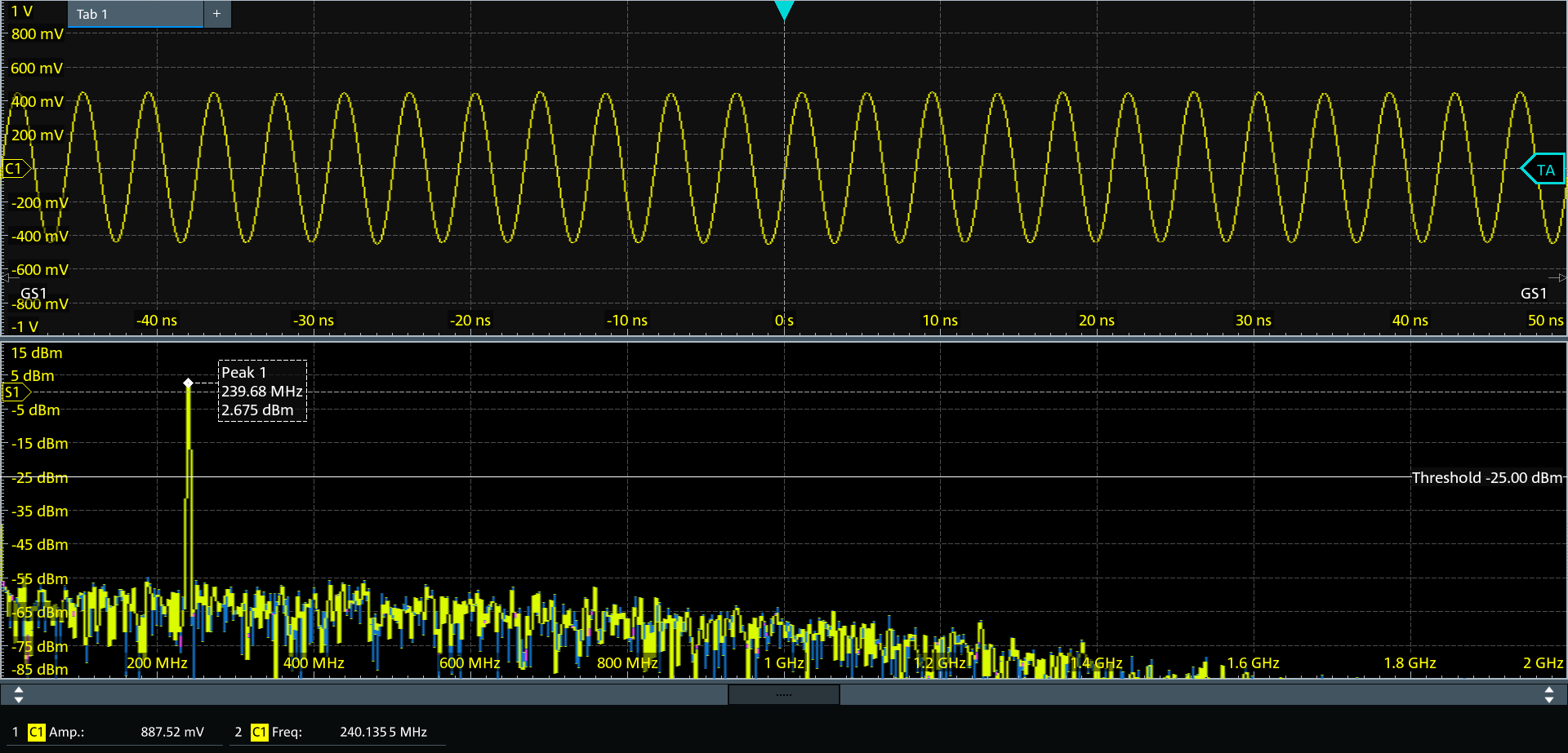
If you connect port 1 of Presto to a low-pass filter VLFX-2500+ and then to the input of an oscilloscope, you should be able to measure something similar to the image below. The amplitude of the 240 MHz tone will depend on the analog configuration of your Presto. In the top panel we see the time domain measurement, and in the bottom panel an FFT of the measured data showing one peak, as expected.

Output multiple tones on one output
In order to output multiple tones, all we need to do is change the parameters of the measurement to include multiple tones. All the rest of the code stays the same. As an example, let’s now output 3 tones.
Note
We’ll use the diff syntax below to mark which lines of code should be added, removed or left unchanged. Like this:
  this line should remain unchanged
- this line should be removed
+ this line should be added
We just need to change the settings for the output group:
-    og = lck.add_output_group(OUTPUT_PORT, 1)
+    og = lck.add_output_group(OUTPUT_PORT, 3)
-    og.set_frequencies(0.0)
+    og.set_frequencies([100e6, 0.0, 50e6])
-    og.set_amplitudes(1.0)
+    og.set_amplitudes([0.2, 0.5, 0.3])
-    og.set_phases(0.0, 0.0)
+    phases_i = [np.pi/4, 0.0, np.pi/2]  # rad
+    phases_q = [3*np.pi/4, -np.pi/2, 0.0]  # rad, +π/2 for LSB, -π/2 for USB
+    og.set_phases(phases_i, phases_q)

     lck.apply_settings()
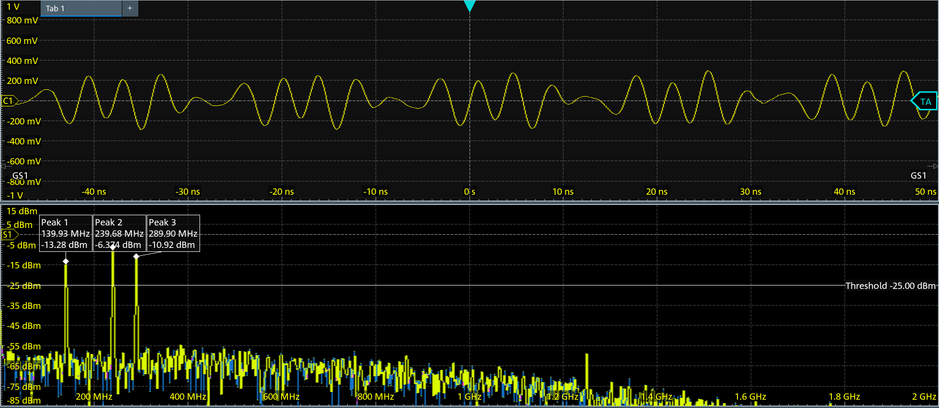
In this example we output tones at:
140 MHz with amplitude 0.2 and phase π/4
(100 MHz IF and lower sideband becausephase_q = phase + np.pi/2)240 MHz with amplitude 0.5 and phase 0
(special case where IF frequency is 0 Hz)290 MHz with amplitude 0.3 and phase π/2
(50 MHz IF and upper sideband becausephase_q = phase - np.pi/2)
Tip
You can learn more about mixers and how phases influence the output at Mixer math.
Note
The amplitude of all the tones on one output should not exceed 1.0 at any point in time. A safe,
conservative way to achieve this is to make sure the sum of all amplitudes doesn’t exceed 1.
Keeping the same cable setup as above, you should be able to measure on your oscilloscope something similar to the image below. The amplitudes of the different tones will again depend on the analog configuration of your Presto. In the top panel, we see the time domain measurement, and in the bottom panel the FFT of the measured data showing three peaks, as expected.

Output multiple tones on multiple outputs
In order to output tones on multiple output ports at the same time, we need to add the parameters for the second port.
  OUTPUT_PORT = 1  # 1 to 16, can be a list
+ OUTPUT_PORT_2 = 2

  LO_FREQ = 240e6  # Hz, LO frequency
+ LO_FREQ_2 = 400e6
We first add the hardware-related parameters:
     lck.hardware.set_dac_current(OUTPUT_PORT, 40_500)  # μA, 2250 to 40500
     lck.hardware.set_inv_sinc(OUTPUT_PORT, 0)
+    lck.hardware.set_dac_current(OUTPUT_PORT_2, 40_500)
+    lck.hardware.set_inv_sinc(OUTPUT_PORT_2, 0)

     lck.hardware.configure_mixer(LO_FREQ, out_ports=OUTPUT_PORT)
+    lck.hardware.configure_mixer(LO_FREQ_2, out_ports=OUTPUT_PORT_2)
Then we add another output group:
     og = lck.add_output_group(OUTPUT_PORT, 1)
     og.set_frequencies([100e6, 0.0, 50e6])
     og.set_amplitudes([0.2, 0.5, 0.3])
     phases_i = [np.pi/4, 0.0, np.pi/2]  # rad
     phases_q = [3*np.pi/4, -np.pi/2, 0.0]  # rad, +π/2 for LSB, -π/2 for USB
     og.set_phases(phases_i, phases_q)

+    og_2 = lck.add_output_group(OUTPUT_PORT_2, 1)
+    og_2.set_frequencies(0.0)
+    og_2.set_amplitudes(1.0)
+    og_2.set_phases(0.0, 0.0)

     lck.apply_settings()
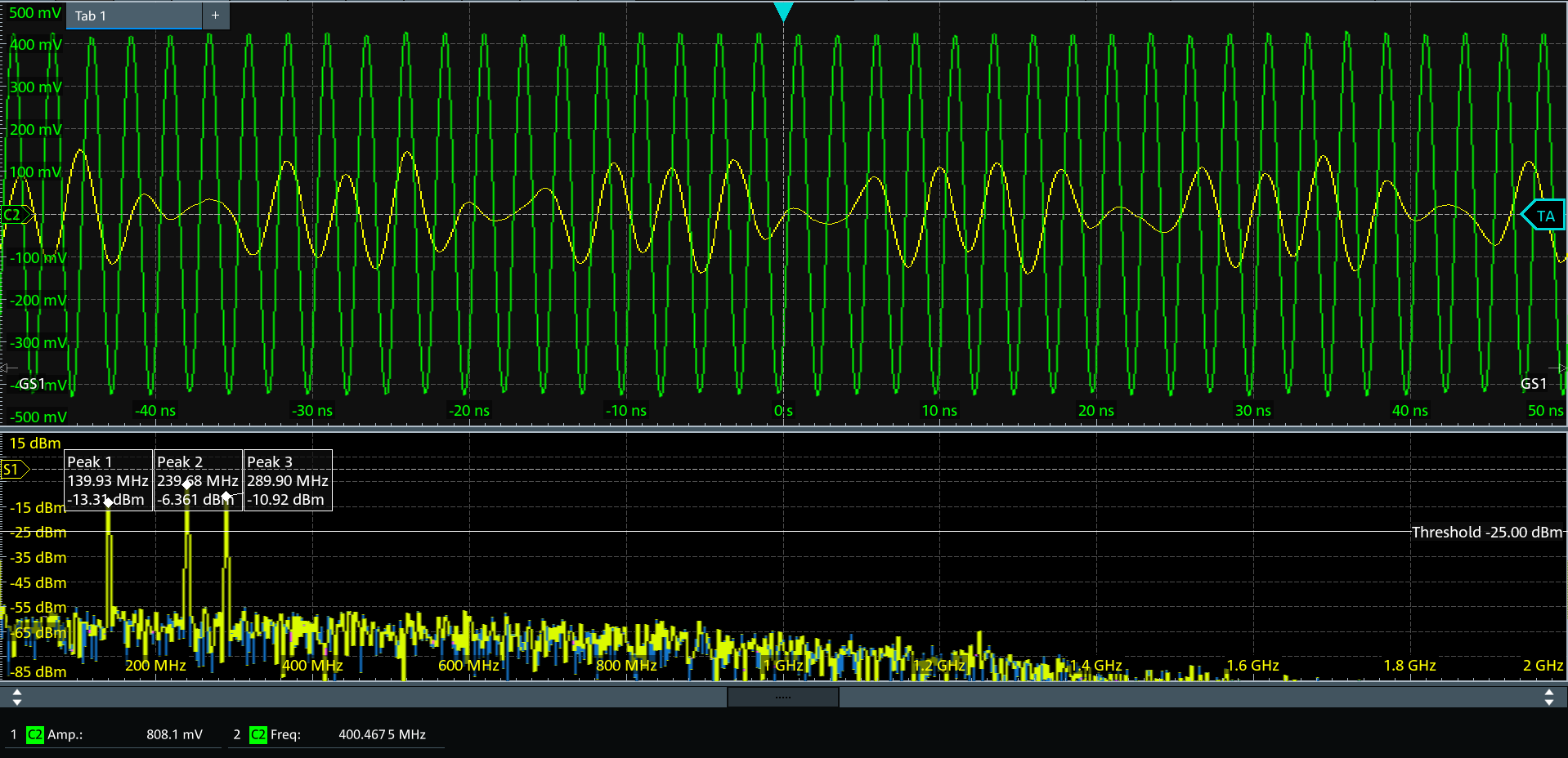
With these settings, we output 3 tones on port 1 (140 MHz, 240 MHz and 290 MHz) just like before, and an additional tone on port 2 at the carrier frequency 400 MHz.
Keep output port 1 Presto connected to one input of the oscilloscope, and now also connect output port 2 of Presto to a second input port of your oscilloscope (through a VLFX-2500+ low-pass filter). You should be able to measure something similar to the image below. In the top panel we see the time-domain measurement of port 1 in yellow and port 2 in green. In the bottom panel we have an FFT of the three tones measured from output 1. The green 400 MHz tone is measured only in time domain to keep all the information in the panels clear.

Measure one tone
Similarly to output groups, there are InputGroups that can be defined on an input
channel. Let’s start by choosing an input port:
  OUTPUT_PORT = 1  # 1 to 16, can be a list
  OUTPUT_PORT_2 = 2
+ INPUT_PORT = 1

  LO_FREQ = 240e6  # Hz, LO frequency
  LO_FREQ_2 = 400e6
We then define configure the hardware settings:
+    lck.hardware.set_adc_attenuation(INPUT_PORT, 0.0)  # dB, 0.0 to 27.0
     lck.hardware.set_dac_current(OUTPUT_PORT, 40_500)  # μA, 2250 to 40500
     lck.hardware.set_inv_sinc(OUTPUT_PORT, 0)
     lck.hardware.set_dac_current(OUTPUT_PORT_2, 40_500)
     lck.hardware.set_inv_sinc(OUTPUT_PORT_2, 0)

-    lck.hardware.configure_mixer(LO_FREQ, out_ports=OUTPUT_PORT)
+    lck.hardware.configure_mixer(LO_FREQ, out_ports=OUTPUT_PORT, in_ports=INPUT_PORT)
     lck.hardware.configure_mixer(LO_FREQ_2, out_ports=OUTPUT_PORT_2)
we disable the input attenuation (0 dB) and setup the input
digital mixer to have the same local-oscillator frequency as the first output port. It is also
possible to setup a different frequency for the input mixer by passing only the in_ports
argument.
We add an input group on the input port and the number of
frequencies we want (one in this case), at what intermediate frequencies we want to measure.
+    ig = lck.add_input_group(INPUT_PORT, 1)  # port, number of frequencies
+    ig.set_frequencies(0.0)  # Hz

     lck.apply_settings()
As soon as we apply the settings, Presto starts to both output and measure tones at the configured frequencies. In our case, it is measuring at 240 MHz on input port 1, and outputting that same frequency from output port 1 (remember that we are still outputting a total of 3 frequencies from port 1 and one more from port 2).
We can request a number of measured data points by calling get_pixels():
     lck.apply_settings()

+    pixel_dict = lck.get_pixels(100)
+    freq_arr, pixel_i, pixel_q = pixel_dict[INPUT_PORT]
The returned pixel_dict is a dictionary where the key is the input port, and the value is a tuple
of three NumPy arrays:
the measured IF frequencies
freq_arr, just[0.0]in this first example;the lockin measurements on the I port of the digital downconversion mixer,
pixel_i;the lockin measurements on the Q port of the digital downconversion mixer,
pixel_q.
Both pixel_i and pixel_q are in principle complex valued. However, in this first example the IF
frequency is zero and so the imaginary part is zero.
We can plot the mean value of the 100 measured points:
fig, ax = plt.subplots(tight_layout=True, figsize=(6, 2.5))
ax.plot(LO_FREQ * 1e-6, np.mean(pixel_i), "b.", label="re")
ax.plot(LO_FREQ * 1e-6, np.mean(pixel_q), "r.", label="im")
ax.legend()
ax.set_xlabel("Frequency (MHz)")
ax.set_ylabel("Amplitude (FS)")
plt.show()
Connect together Presto’s output port 1 and input port 1, through the VLFX-2500+ low-pass filter. You should then be able to measure something similar to the image below. Since we plot the real and the imaginary components of the lockin measurement, your measured values can differ based on the length of your cables and the analog configuration of your Presto.
Measure multiple tones
To measure multiple tones, we simply add more frequencies to the input group:
-    ig = lck.add_input_group(INPUT_PORT, 1)  # port, number of frequencies
+    ig = lck.add_input_group(INPUT_PORT, 2)  # port, number of frequencies
-    ig.set_frequencies(0.0)  # Hz
+    ig.set_frequencies([0.0, 50e6])  # Hz

     lck.apply_settings()
The rest of the code is identical. The only difference is in plotting the data, as now we have 2
frequencies to plot. Moreover, one of the frequencies is nonzero, so we have to pay attention if we
want to plot the upper sideband (USB) or the lower sideband (LSB). Presto always measures both
sidebands, and the function utils.untwist_downconversion() helps us to extract the LSB and
USB individually from the IQ data:
     pixel_dict = lck.get_pixels(100)
     freq_arr, pixel_i, pixel_q = pixel_dict[INPUT_PORT]
+    lsb, usb = untwist_downconversion(pixel_i, pixel_q)
Since we output only the USB (at 290 MHz), we plot just the USB:
  fig, ax = plt.subplots(tight_layout=True)
- ax.plot(LO_FREQ * 1e-6, np.mean(pixel_i), "b.", label="re")
- ax.plot(LO_FREQ * 1e-6, np.mean(pixel_q), "r.", label="im")
+ ax.plot((LO_FREQ + freq_arr) * 1e-6, np.mean(np.real(usb), axis=0), "C0o", label="re")
+ ax.plot((LO_FREQ + freq_arr) * 1e-6, np.mean(np.imag(usb), axis=0), "C1o", label="im")
  ax.legend()
  ax.set_xlabel("Frequency (MHz)")
  ax.set_ylabel("Amplitude (FS)")
  plt.show()
Turn off the outputs
To turn-off the outputs at the end of the experiment, we set the amplitude to zero in both output groups, and then apply the settings:
    og.set_amplitudes(0)
    og_2.set_amplitudes(0)
    lck.apply_settings()
Complete code
If you made it this far and applied all the code changes of the previous sections, congratulations! You probably have in front of you a script that looks like the one below here. Keep in mind that you can also have a look at the various example scripts in the presto-demo repository.
from matplotlib import pyplot as plt
import numpy as np

from presto import lockin
from presto.hardware import AdcMode, DacMode
from presto.utils import untwist_downconversion

OUTPUT_PORT = 1  # 1 to 16, can be a list
OUTPUT_PORT_2 = 2
INPUT_PORT = 1

LO_FREQ = 240e6  # Hz, LO frequency
LO_FREQ_2 = 400e6

with lockin.Lockin(
    address="192.168.20.23",
    ext_ref_clk=False,
    adc_mode=AdcMode.Mixed,
    dac_mode=DacMode.Mixed,
) as lck:
    lck.hardware.set_adc_attenuation(INPUT_PORT, 0.0)  # dB, 0.0 to 27.0
    lck.hardware.set_dac_current(OUTPUT_PORT, 40_500)  # μA, 2250 to 40500
    lck.hardware.set_inv_sinc(OUTPUT_PORT, 0)
    lck.hardware.set_dac_current(OUTPUT_PORT_2, 40_500)
    lck.hardware.set_inv_sinc(OUTPUT_PORT_2, 0)

    lck.hardware.configure_mixer(LO_FREQ, out_ports=OUTPUT_PORT, in_ports=INPUT_PORT)
    lck.hardware.configure_mixer(LO_FREQ_2, out_ports=OUTPUT_PORT_2)

    lck.set_df(1e3)

    og = lck.add_output_group(OUTPUT_PORT, 3)  # port, number of frequencies
    og.set_frequencies([100e6, 0.0, 50e6])  # Hz, IF frequency
    og.set_amplitudes([0.2, 0.5, 0.3])  # full-scale units, output amplitude, 0.0 to 1.0
    phases_i = [np.pi / 4, 0.0, np.pi / 2]  # rad
    phases_q = [3 * np.pi / 4, -np.pi / 2, 0.0]  # rad, +π/2 for LSB, -π/2 for USB
    og.set_phases(phases_i, phases_q)

    og_2 = lck.add_output_group(OUTPUT_PORT_2, 1)
    og_2.set_frequencies(0.0)
    og_2.set_amplitudes(1.0)
    og_2.set_phases(0.0, 0.0)

    ig = lck.add_input_group(INPUT_PORT, 2)  # port, number of frequencies
    ig.set_frequencies([0.0, 50e6])  # Hz

    lck.apply_settings()

    pixel_dict = lck.get_pixels(100)
    freq_arr, pixel_i, pixel_q = pixel_dict[INPUT_PORT]
    lsb, usb = untwist_downconversion(pixel_i, pixel_q)

    og.set_amplitudes(0)
    og_2.set_amplitudes(0)
    lck.apply_settings()


fig, ax = plt.subplots(tight_layout=True, figsize=(6, 2.5))
ax.plot((LO_FREQ + freq_arr) * 1e-6, np.mean(np.real(usb), axis=0), "C0o", label="re")
ax.plot((LO_FREQ + freq_arr) * 1e-6, np.mean(np.imag(usb), axis=0), "C1o", label="im")
ax.legend()
ax.set_xlabel("Frequency (MHz)")
ax.set_ylabel("Amplitude (FS)")
plt.show()